Sklearn data Pre-Processing using Standard and Minmax scaler

In Machine learning the variables that are measured at different scales can impact the numerical stability and precision of the estimators

Some of the Machine Learning estimators may behave in-appropriately if the features have different ranges. For example, Salary in range 50K-150K and Age in range 32-68 years

Data Standardization is the process of putting different variables on the same scale. This process allows you to compare scores between different types of variables

In this post we will see how sklearn.preprocessing module is used for scaling, centering, normalization and Transforming data

We will discuss two methods for sklearn.preprocessing i.e., Standard scaler and MinMaxScaler in this post and will briefly touch on other methods as well

Standard Scaler

Using StandardScaler function of sklearn.preprocessing we are standardizing and transforming the data in such a way that the mean of the transformed data is 0 and the Variance is 1

The fit() method is used to compute the mean and std dev which will be used for later scaling. This method computes it separately for each feature in a dataset

Next Transform method is used to perform Standardization by centering and Scaling.

So fit_transform() method can be used on Train set for computing the mean and std for each feature and then transform() can be later used on with the Test data set

Let’s look at an example on how it works

Create a 2D matrix with random integers with range [-1,3]

from sklearn import preprocessing
import numpy as np
X_train = np.random.randint(-1,3, size=(3, 3))
X_train

array([[-1, -1, -1],
       [ 0,  1,  2],
       [ 0, -1, -1]])

Create an Object of StandardScaler

scaler = preprocessing.StandardScaler()

StandardScaler(copy=True, with_mean=True, with_std=True)

We will use fit() function to compute the mean, variance and std dev of the X_train along axis = 0

scaler.fit(X_train)
print('  mean: ',scaler.mean_,'n','variance: ',scaler.var_)

mean:  [-0.33333333 -0.33333333  0. ]
variance:  [0.22222222 0.88888889 2. ]

Now transform the X-train data to remove the mean and scale Variance to 1

scaler.transform(X_train)

array([[-1.41421356, -0.70710678, -0.70710678],
       [ 0.70710678,  1.41421356,  1.41421356],
       [ 0.70710678, -0.70710678, -0.70710678]])

This is finally the transformed data using the Standardscaler with mean Zero and Standard Deviation and Variance of 1

Let’s use the preprocessing scale() function to transform the same dataset and see if it gives the same result or not

X_transformed = preprocessing.scale(X_train)

array([[-1.41421356, -0.70710678, -0.70710678],
       [ 0.70710678,  1.41421356,  1.41421356],
       [ 0.70710678, -0.70710678, -0.70710678]])

So we get the same result here as well. Let’s check the mean and Variance of the transformed data

print(' Mean:  ',X_transformed.mean(axis=0),'n','Stdev: ',X_transformed.std(axis=0))

Mean:   [-7.40148683e-17 -7.40148683e-17  0.00000000e+00]
Stdev:  [1. 1. 1.]

The mean and Stdev along axis = 0 is zero and one respectively so the data is standardized appropriately

Let’s try the same scaler on a New dataset

X_test = np.random.randint(-1,3, size=(2,3))
X_test

array([[1, 2, 2],
       [2, 1, 2]])

Now use the same scaler instance as above and transform this new or test dataset the same way as it did it for X_train

scaler.transform(X_test)

array([[-1.41421356,  2.47487373,  1.33630621],
       [ 0.70710678,  1.41421356,  1.33630621]])

MinMax Scaler

It standardize the data by transforming within a given range. Moreover the Feature scaling lies between a minimum and maximum value so that the maximum absolute value of each feature is scaled to unit size

Minmaxscaler also scales each of the feature individually for example between 0 and 1. This is good scaling options when you want to preserve the zero’s in a sparse dataset

Following formula is used for the transformation

X_std = (X - X.min(axis=0)) / (X.max(axis=0) - X.min(axis=0))
X_scaled = X_std * (max - min) + min

Let’s see how it works for a small dataset. We will use the X_train dataset from above

We will scale X_train to a range [0,3]. The feature_range param used for setting up the desired range of transformed data

The fit_transform method fits to data and then transforms it

min_max_scaler = preprocessing.MinMaxScaler(feature_range=(0, 3))
X_train_minmax = min_max_scaler.fit_transform(X_train)
X_train_minmax

We can use the same instance of min_max_Scaler on the X_test dataset created above

X_test_minmax = min_max_scaler.transform(X_test)
X_test_minmax

array([[ 3. ,  0. ,  3. ],
       [ 4.5, -3. ,  3. ]])

Use scale_ attribute to check the min_max_scaler attributes to determine the exact nature of the transformation learned on the training data

The scale_ attribute is Per feature relative scaling of the data. Equivalent to (max - min) / (X.max(axis=0) - X.min(axis=0))

Let’s check the scale_ attributes that is learnt for our example

min_max_scaler.scale_

array([1.5, 1.5, 1. ])

There is another function min_max_scale which is an equivalent function without the estimator API

Real World Dataset

Let’s work on real dataset and check how standard and min_max scaling works on features of sklearn wine dataset

from sklearn.datasets import load_wine
windata = load_wine()

Features of Wine dataset

windata.feature_names

['alcohol',
 'malic_acid',
 'ash',
 'alcalinity_of_ash',
 'magnesium',
 'total_phenols',
 'flavanoids',
 'nonflavanoid_phenols',
 'proanthocyanins',
 'color_intensity',
 'hue',
 'od280/od315_of_diluted_wines',
 'proline']

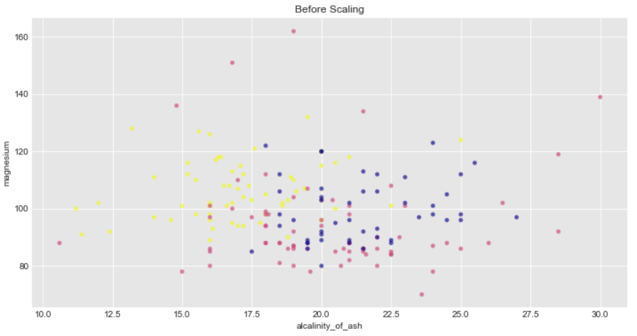
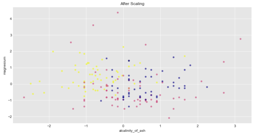
We will consider only features alcalinity_of_ash and magnesium for scaling and standardization since there are outliers available in these features

X = windata.data[:,[3,4]]
y = windata.target
# scale the output between 0 and 1 for the colorbar
y = minmax_scale(y)

Let’s do a StandardScaler transform of the features

X_transform = StandardScaler().fit_transform(X)

We will plot the data with their target data(Y) as colormaps in a 2D axis

Additionally Standard scalar removes the mean therefore the spread of transformed data for each feature is different. Transformed alcalinity_of_ash has a range of [-2,3] whereas transformed magnesium is squeezed in [-2,4]

%matplotlib inline
import matplotlib.pyplot as plt
import matplotlib as mpl
import seaborn as sns
sns.set_style("darkgrid", {"axes.facecolor": ".9"})

from matplotlib import cm

The scatter plot

fig, (ax1,ax2) = plt.subplots(1, 2,figsize=(20,6))
colors = cmap(y)
ax2.scatter(X_transform[:, 0], X_transform[:, 1], alpha=0.5, marker='o', s=10, lw=2, c=colors)
ax1.scatter(X[:, 0], X[:, 1], alpha=0.5, marker='o', s=10, lw=2, c=colors)
ax1.set_title("Before Scaling")
ax2.set_title("After Scaling")

You can explore the minmax Standardization on wine dataset on your own and check how far each of the features squeezed in

Other Preprocessing scalers, transformers, and normalizers

The scope of this post is only limited to evaluate minmax and standard scaler. I will briefly touch upon other methods that are available and can be explored for normalization or standardization of data.

This is not a complete list but a subset

1. preprocessing.MaxAbsScaler: Scales each feature by its maximum absolute value. It does not shift/center the data, and therefore does not destroy any sparsity
2. preprocessing.Normalizer: Normalize samples features individually to unit norm. it is mostly used for text classification or clustering for instance
3. preprocessing.PowerTransformer: Apply a power transform on features to make it Gaussian like. Common methods are Box-Cox and Yeo-Johnson transform(if data contains negatives)
4. preprocessing.QuantileTransformer: It transform features using Quantiles to follow a uniform and normal distribution

Conclusion:

Here are the key takeways and summary of this entire post:

• Sklearn preprocessing module is used for Scaling, Normalization and Standardization of the data
• StandardScaler removes the mean and scales the variance to unit value
• Minmax scaler scales the features to a specific range often between zero and one so that the maximum absolute value of each feature is scaled to unit size
• Maxabs scaler scales in a way that the training data lies within the range [-1,1] by dividing each data point with the max value. Assumption is that the data is already centered to Zero
• Power transformer is used to transform the data into Normal distribution like and it is a type of Non linear transform method
• Moreover Box cox is used for only positive dataset and if there are negatves in the data then preferred power transform method is Yeo-Johnson transform
• Normalization is often used in text classification and clustering contexts. It is the process of scaling the data samples to unit norm
• Quantile Transform is a type of Non-linear transform and transforms data to follow a unform or normal distribution