Decision Tree in Sklearn
In this post we are going to see how to build a basic decision tree classifier using scikit-learn package and how to use it for doing multi-class classification on a dataset.
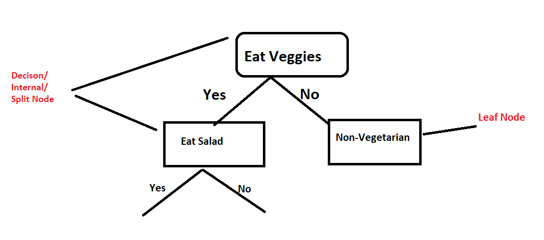
Decision trees is an efficient and non-parametric method that can be applied either to classification or to regression tasks.
To predict the dependent variable the input space is split into local regions because they are hierarchical data structures for supervised learning
Decision tree is a simple to learn and easy to interpret and Visualize the decisions in a tree format. It has the advantage of producing comprehensible classification/regression model with satisfactory accuracy level.
We will be exploring the DecisionTreeClassifier function of sklearn and all the parameters of it. You will also see how to Visualize the decision tree Rules and the Boundaries that model is creating to classify the different Classes(targets)
Decision Tree Classifier in Sklearn
sklearn.tree.DecisionTreeClassifier(_criterion='gini'_, _splitter='best'_, _max_depth=None_,

_min_samples_split=2_, _min_samples_leaf=1_, _min_weight_fraction_leaf=0.0_, _max_features=None_,

_random_state=None_, _max_leaf_nodes=None_, _min_impurity_decrease=0.0_, _min_impurity_split=None_,

_class_weight=None_,  _ccp_alpha=0.0_)
Parameters
criterion
Gini or entropy and default is Gini.
One of the Critical factor is to choose which feature for splitting the nodes in subsets and for making that decision we choose out of these two criteria
- Information Theory (Entropy)
- Distance Based (Gini)
Both are impurity measures and it looks like the selection of impurity measure has little effect on the performance of single decision tree algorithms
The impurity is measured before and after splitting a node according to each possible attribute.
The attribute which presents the greater gain in purity, i.e., that maximizes the difference of impurity taken before and after splitting the node, is chosen
Entropy might be a little slower to compute because it makes use of the logarithm
Splitter
Strategy to choose out of best or random. Default is best
If the best strategy is chosen then it will split on the most important feature first
it will choose a feature on random for splitting the node if splitter set to random which could lead to accuracy and more depth in the decision tree
max_depth
The maximum depth of the tree.
One of the stopping criteria that let you decide when to terminate the tree building process. A tree can be grown until a maximum depth is reached.
A tree can be grown to a maximum depth of N-1 where N is the number of samples
Beside max_depth there are other stopping criteria as well so in reality a tree will never go a maximum depth of N-1
Mostly we try to pick the optimal depth based on cross-validation and decides the reasonable max_depth value
min_samples_split
The minimum number of samples required at an Internal node for splitting. Say for example min_samples_split = 5 and there are 8 samples at a decision node then the split is allowed otherwise if <5 then not allowed.
if min_sample_leaf = 2 and one leaf has 1 sample and other has 6 samples then the split is not allowed
so min_samples_split depends on the min-sample_leaf defined as well

min_samples_leaf
The minimum number of samples required at a leaf node
min_weight_fraction_leaf
The minimum weighted fraction
`fit`(_self_, _X_, _y_, _sample_weight=None_, _check_input=True_, _X_idx_sorted=None_)
this parameter decides the required fraction of samples (or weights) in each leaf node
It uses the weight defined for each sample thru the fit method that has a sample_weight which lets you specify the weight of each of the samples and accepts values in an array like format for n_samples
if a minimum weight fraction is set and the sample weight is None then it will assume a uniform weight for all the samples
max_features
It defines the number of features to be used for best split.
It is used to control the over-fitting. For example if the shape of your data is 30 and max_feature is set to 5.
So Every time at a decision node you will choose maximum of 5 features that are selected randomly for splitting
random_state
It is the seed used by the random number generator. it is basically used to make the result or outcome of the classifier consistent.
It hardly matters what number you select but if you select the same number each time then the output remains deterministic
max_leaf_node
maximum leaf node. It is one of the stopping criteria to grow a tree wih max_leaf_node.
By default it is set to None which means it will grow to unlimited leaf nodes and other stopping criteria will be considered
from the official documentation the formula for weighted impurity decrease is as follows:
N_t / N * (impurity - N_t_R / N_t * right_impurity
                    - N_t_L / N_t * left_impurity)
This formula takes into account how much the parent node makes up of the total tree (N_t / N) and the weighted impurity decrease from the child nodes.
If the final impurity decrease is less than the minimum impurity decrease parameter, then the split will not be performed
class_weight
By default all the classes have same weight i.e. 1
The class_weight parameter deals well with unbalanced classes by giving more weight to the under represented classes.
It is used for re-weighting the splitting criterion
Higher the class_weight more you want to put emphasis on that class.
For multi-output, class_weights will be multiplied with sample_weight (passed through the fit method) if sample_weight is specified
Get Started
We will use the wine dataset from sklearn.
Let’s load the data and then will split into train and test sets
from sklearn import datasets
from sklearn.tree import DecisionTreeClassifier
wine_data = datasets.load_wine()
Let’s check out the important keys in this dataset
wine_data.keys()
dict_keys(['data', 'target', 'target_names', 'DESCR', 'feature_names'])
So we have data, target variables with their names stored in target_names and feature names
Let’s find out the features in the data that we will use to train the decision tree classifier
wine_data.feature_names
['alcohol',
 'malic_acid',
 'ash',
 'alcalinity_of_ash',
 'magnesium',
 'total_phenols',
 'flavanoids',
 'nonflavanoid_phenols',
 'proanthocyanins',
 'color_intensity',
 'hue',
 'od280/od315_of_diluted_wines',
 'proline']
Here are the different classes or targets in which each of these data is classified to i.e. class_0, class_1 and class_2
wine_data.target_names
**array(['class_0', 'class_1', 'class_2'], dtype='<U7')**
Finally lets check the data by importing it into a Dataframe object. So you can visualize how the data looks like
import pandas as pd
pd.DataFrame(wine_data.data,columns=wine_data.feature_names)
We can see there are 178 rows and 13 features in this dataset.

Train Test Split
We have split the data into training and test set using sklearn train_test_split
from sklearn.model_selection import train_test_split
X_train, X_test, y_train, y_test = train_test_split(X, y, test_size=0.3,
stratify=y)
Accuracy Score and Cross Validation
Lets measure the testing accuracy using sklearn accuracy_score.
For that we are going to instantiate the Decision tree classifier and then use the fit method on Train data.
Predict method of decision tree classifier will find the target class for the test data
Finally we will calculate the accuracy on our test data prediction
from sklearn.metrics import accuracy_score

clf = DecisionTreeClassifier() #Instantiate Decision tree classifier
clf.fit(X_train, y_train)      # Use fit method on the train data

y_pred = clf.predict(X_test)   # Predict the target class of test data
accuracy_score(y_test, y_pred)  # Measure Accuracy
Let’s evaluate the cross validation score as well
from sklearn.model_selection import cross_val_score
scores = cross_val_score(clf, X_test, y_test, cv=5)
print("Accuracy: %0.2f (+/- %0.2f)" % (scores.mean(), scores.std() * 2))
Visualize Decision Tree using plot_tree
You can also Visualize the final decision tree by using the plot_tree function of the sklearn.
There are other ways to visualize using pydot and graphviz but I’m not going to discuss those methods in this post
%matplotlib inline
from matplotlib.pyplot import figure
from sklearn.tree import plot_tree
figure(num=None, figsize=(20, 6), dpi=80, facecolor='w', edgecolor='k')
plot_tree(clf.fit(wine_data.data, wine_data.target))

GridSearchCV
Hyper parameters selection is an important part for model selection. how would you know what combinations of these parameters will give you the best outcome?
One way is randomly selecting these values and see which combinations of parameters will give best result.
Isn’t that tedious to do? So Grid Search in Scikit-learn exactly does the same thing and helps to find the best estimator
from sklearn.model_selection import GridSearchCV, cross_val_score
param_grid = {'criterion':['gini','entropy'], 'max_depth' :
[3,5,7,20]}
grid_search = GridSearchCV(clf,param_grid=param_grid,cv=5)
grid_search.fit(X_train, y_train)

You can see all the criteria and their respective score that gridsearch used to evaluate the best estimate by accessing the params and mean_test_score of grid search object
The params and the mean_test_score keys will give you the parameters and their corresponding results
grid_search.cv_results_['params']
grid_search.cv_results_['mean_test_score']
([{'criterion': 'gini', 'max_depth': 3},
  {'criterion': 'gini', 'max_depth': 5},
  {'criterion': 'gini', 'max_depth': 7},
  {'criterion': 'gini', 'max_depth': 20},
  {'criterion': 'entropy', 'max_depth': 3},
  {'criterion': 'entropy', 'max_depth': 5},
  {'criterion': 'entropy', 'max_depth': 7},
  {'criterion': 'entropy', 'max_depth': 20}],
 array([0.89466667, 0.878     , 0.88666667, 0.87866667, 0.93533333,
        0.91933333, 0.93533333, 0.91933333]))
Get Best Estimator
We will use the best_estimator_ attribute to find the best combination of these parameters for our wine dataset
grid_search.best_estimator_

Just check it out if using the best estimator improves the above accuracy_score or not
from sklearn.metrics import accuracy_score
y_pred_gs = grid_search.predict(X_test)
accuracy_score(y_test, y_pred_gs)
Decision Surface of Decision Tree
Let’s do some additional visualization of the decision tree to understand how decision tree classify between two classes using 2D plot between any of the two features here
We will plot the decision surface of a decision tree trained on pairs of features of the wine dataset
We are creating a numpy meshgrid to plot the decision boundary by predicting it’s classes and plotting a contour
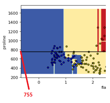
Look at those two plots below between proline & flavanoids and proline & od280. You can see those horizontal lines created by decision tree to classify the three different classes of the wine
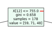
if you see the tree structure above that we have created it is splitting at feature 12 i.e., proline at value 755

Because we have drawn a horizontal line in the below plot at y=755 it shows the exact line that divides the two rectangles representing the two classes i.e., class_0 and class_1

So this decision boundary visualization gives you the idea exactly how the decision tree is making decisions on differentiating the classes using the features and you can also co-relate this with the tree
We only take the two corresponding features
import numpy as np
import matplotlib.pyplot as plt
from matplotlib.pyplot import figure
from sklearn.tree import plot_tree
figure(num=None, figsize=(20, 6), dpi=80, facecolor='w', edgecolor='k')

#parameters
pair = [11,12]
pairidx = 0
n_classes = 3
plot_colors = "ryb"
plot_step = 0.02

X = wine_data.data[:, pair]
y = wine_data.target

# Train
clf = gs_inst.best_estimator_.fit(X, y)

# Plot the decision boundary
plt.subplot(2, 3, pairidx + 1)

x_min, x_max = X[:, 0].min() - 1, X[:, 0].max() + 1
y_min, y_max = X[:, 1].min() - 1, X[:, 1].max() + 1
xx, yy = np.meshgrid(np.arange(x_min, x_max, plot_step),
                     np.arange(y_min, y_max, plot_step))
plt.tight_layout(h_pad=0.5, w_pad=0.5, pad=2.5)

Z = clf.predict(np.c_[xx.ravel(), yy.ravel()])
Z = Z.reshape(xx.shape)
cs = plt.contourf(xx, yy, Z, cmap=plt.cm.RdYlBu)

plt.xlabel(wine_data.feature_names[pair[0]])
plt.ylabel(wine_data.feature_names[pair[1]])

# Plot the training points
for i, color in zip(range(n_classes), plot_colors):
    idx = np.where(y == i)
    plt.scatter(X[idx, 0], X[idx, 1], c=color, label=wine_data.target_names[i],
                cmap=plt.cm.RdYlBu, edgecolor='black', s=15)

plt.suptitle("Decision surface of a decision tree using paired features")
plt.legend(loc='lower right', borderpad=0, handletextpad=0)
plt.axis("tight")
plt.axhline(y = 755,
color='black')

plt.figure()
figure(num=None, figsize=(20, 6), dpi=80, facecolor='w', edgecolor='k')
clf = DecisionTreeClassifier().fit(wine_data.data, wine_data.target)
plot_tree(clf, filled=True)
plt.show()
I have just used these two pairs of features to plot this:
- Proline vs od280/od315_of_diluted_wines
- Proline vs Flavanoids
If you want to see the decision boundary for all the possible pairs of 13 features then just run the above code in the loop. You can check the code in the documentation. They have exactly done the same thing


Feature Importance
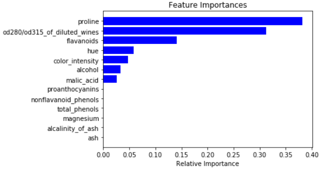
It is one of the important attribute to know the dominant feature for your model. Feature_Importance gives the score for each of the features on how useful they are in predicting the target variable
The feature_importance score is based on how purely a node separates the classes i.e. Gini Index
The importance of a feature is computed as the (normalized) total reduction of the criterion brought by that feature. It is also known as the Gini importance
We will plot all the important features based on their scores evaluated by feature_importance function
For splitting the decision node the most important feature is used as the first attribute
Check the tree visualization above to see the attribute used for splitting
#Feature Importance
importances=clf.feature_importances_

features = wine_data['feature_names']
importances = clf.feature_importances_
indices = np.argsort(importances)

plt.title('Feature Importances')
plt.barh(range(len(indices)), importances[indices], color='b', align='center')
plt.yticks(range(len(indices)), [features[i] for i in indices])
plt.xlabel('Relative Importance')
plt.show()

Extract Decision Tree Rule as a Text Report
We can also export the decision tree rules in a text format. Use export_text function of sklearn tree to achieve that
it provides the same rule that we have visualized in a graphical format above but this seems to be more readable
from sklearn.tree.export import export_text
tree_rules = export_text(clf, feature_names=wine_data.feature_names)
print(tree_rules)

What’s next
Decision tree builds a Regression model and it works pretty much same as the classifier by building the basic tree model for regression. So it will be a good attempt to leverage your learning to build the Decison Tree Regression model and see how the hyper-parameters differs from the classifier model and the final outcome looks like
In the next post we will be discussing about the ensemble methods such as Random Forest and Gradient Boosting Machines algorithm
The main objective of the ensemble tree algorithms is to combine the various base weak models like decision tree and come up with an optimal model for prediction
Conclusion
Here are the points to summarize our learning so far :
- Decision Tree in Sklearn uses two criteria i.e., Gini and Entropy to decide the splitting of the internal nodes
- The stopping criteria of a decision tree: max_depth, min_sample_split and min_sample_leaf
- The class_weight parameter deals well with unbalanced classes by giving more weight to the under represented classes
- The sample_weight lets you specify the weight of each of the samples in the dataset
- We have used sklearn wine dataset with 13 features and 178 observations to build a Decision Tree Classifier
- Accuracy_score function let you know the accuracy on your test set
- Cross-validation for detecting and preventing overfitting
- Visualize the decision tree using the plot_tree in sklearn. Additionally, you can also use pydot and graphviz for visualization too
- For the hyper parameter selection and getting the best estimator for your dataset one can use Grid Search CV
- Another Visualization of Decision surface of decision tree boundaries helps you to understand how the model create boundaries between these classes
- Feature_importance is an Important attribute that gives the dominant feature for your model. It provides the score for each of the features on how useful they are in predicting the target variable
- To export the decision tree rule in text format or report you can use the export_text
You can find all the code used in this post in this github link for jupyter notebook: https://github.com/min2bro/Tree-Based-Algorithms/blob/master/Decision%20Tree%20Classifier%20in%20sklearn.ipynb